Results
Optimisation has been one of the main aspects we have worked on while developing this project. We wanted to deliver a fast, yet accurate simulation. We think we managed to obtain good results, with a full simulation and reconstruction of 1 million events being run in under 2:30 minutes.
Following are the results of $3$ simulations that we ran with different configurations. A comparison between them can be found at the end of the page. Click to display each run results:
❯ Run 1
Configuration:
- N events: 1 million
- Multiplicity distribution: Charged-particle multiplicity measurement in proton-proton collisions at sqrt(s) = 7 TeV with ALICE at LHC
- Angular distribution: uniform
- $Z_{vertex}$ distribution: gaussian
- $\sigma_{x}=0.01$ cm, $\sigma_{y}=0.01$ cm, $\sigma_{z}=5.3$ cm
- Beam pipe radius: $3$ cm
- Detectors radii: $4$cm, $7$cm
- Noise: no
- MaxPhi: 0.01 mrad
- nSigmaZ: 3
Simulation configuration file here. Reconstruction configuration file here.
Simulation
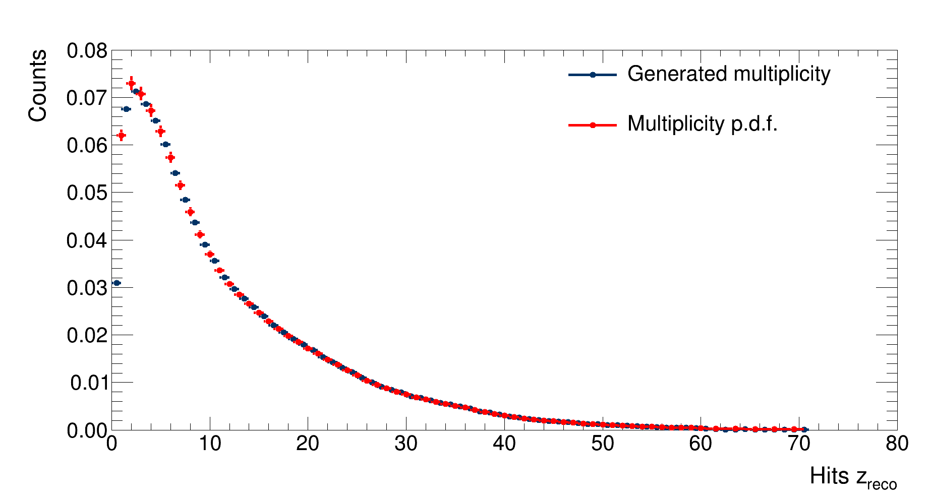
Firstly, this is a comparison between the multiplicity probability density function (pdf) and the (normalised) generated multiplicity distribution:
 |
|---|
| Comparison between the multiplicity pdf and the (normalised) generated multiplicity distribution |
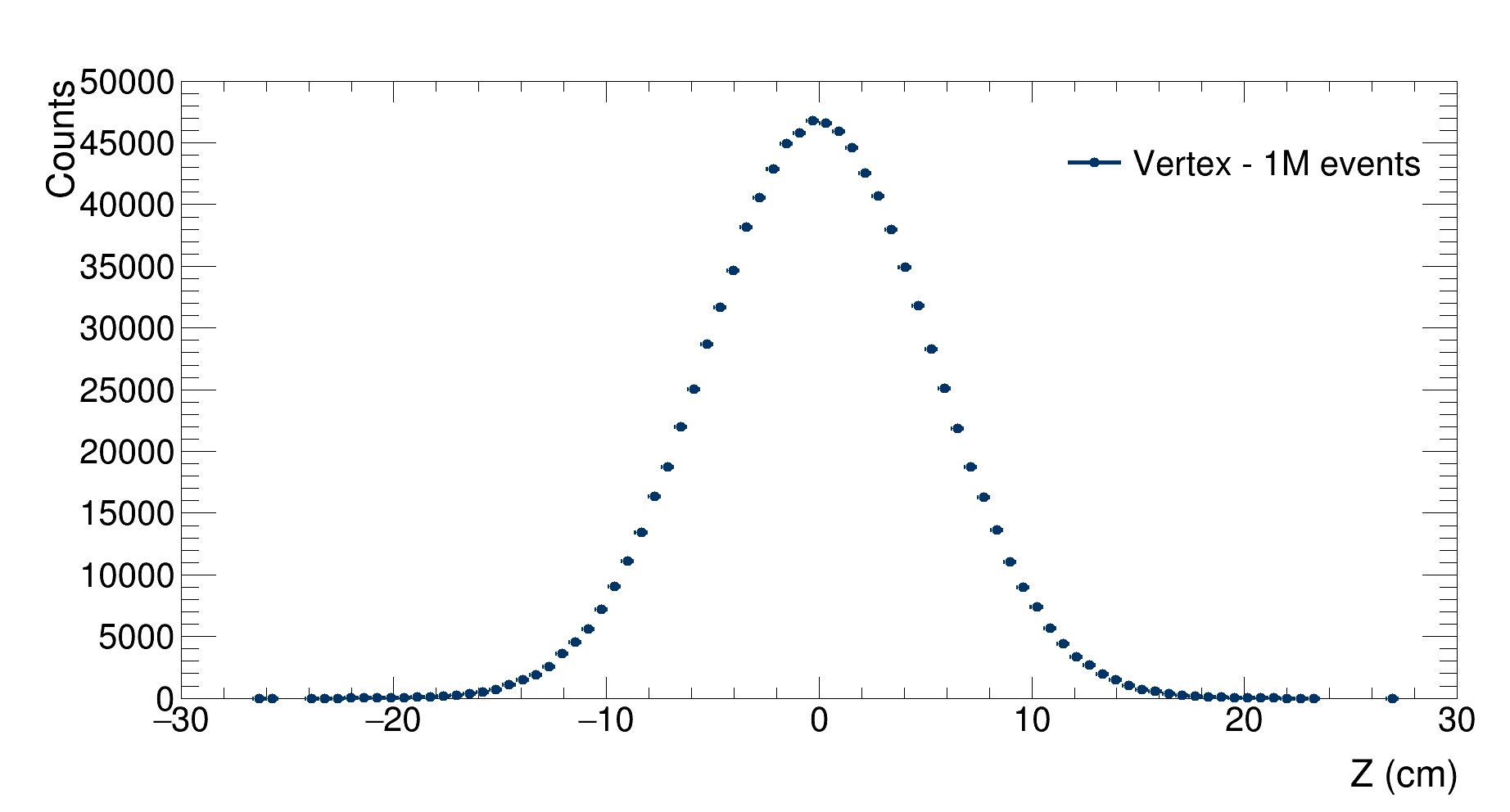
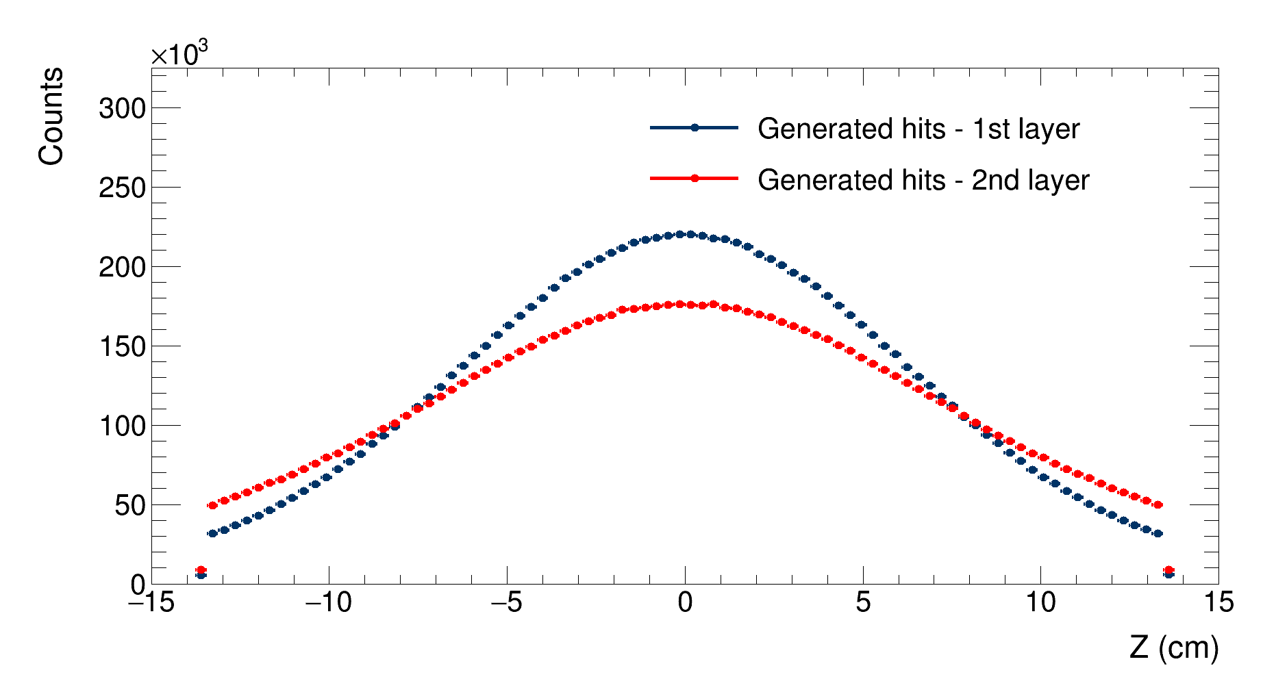
A good agreement between the two distributions is observed. In order to study the effects of the multiple scattering, it is possible to study the difference between the $z$ coordinate distribution of the generated hit in the two layers and the $z$ coordinate pdf of the vertex:
 |
|---|
| Distribution of the generated $z$ coordinate of the vertex. $\mathrm{RMS}=5.3$ cm |
 |
|---|
| Comparison between the distributions of the hits’ $z$ coordinate for the first layer (in blue, $\mathrm{RMS}=6.7$ cm) and the second layer (in red, $\mathrm{RMS}=7.7$ cm) |
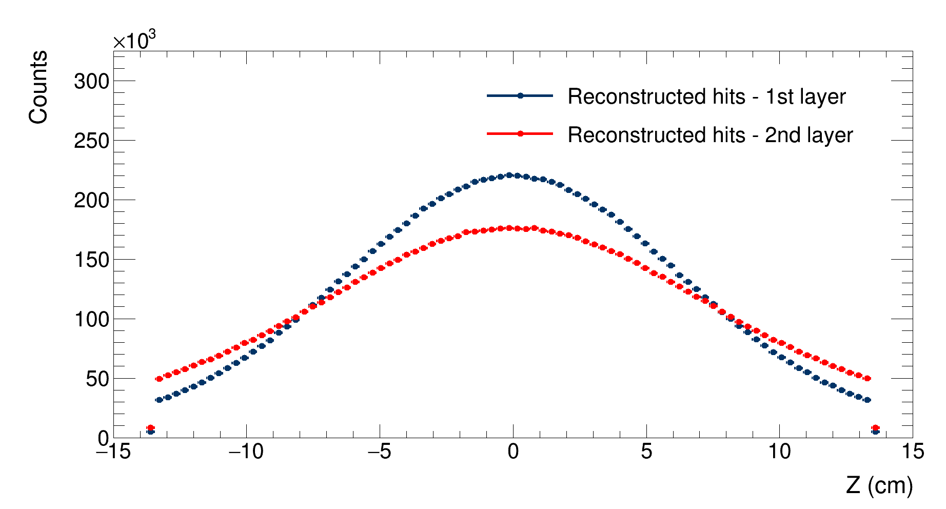
To study how the smearing affects the reconstruction, it is possible to study the distributions of the reconstructed z coordinates of the hits on each detector’s layer:
 |
|---|
| Comparison between the distributions of the reconstructed (smeared) hits’ z coordinate for the first layer (in blue, $\mathrm{RMS}=6.8$ cm) and the second layer (in red, $\mathrm{RMS}=7.4$ cm) |
As expected, smearing does not have any effects on the shape of the distributions, nor does it affects the distributions widths as much as the multiple scattering does.
Reconstruction
After the simulation finishes, vertexes are reconstructed and the resolution and effeciency of the detector are evaluated as a function of the event multiplicity and of the event’s $Z_{vertex}$ coordinate. The efficiency is evaluated as the ratio between the number of reconstructed vertexes and the total number of events; its error is obtained through binomial propagation. The resolution is evaluated as the sum in quadrature of the $\sigma$ of the gaussian function obtained with a maximum likelihood fit of the residuals histogram and the shift from 0 (estimated as the mean of the residuals distribution) in the studied $Z_{vertex}$ and multiplicity range. Its uncertainty is given by the uncertainty on the $\sigma$ parameter of the fitted gaussian. It is needed to take into account the shift of the distribution since for events generated near the detector’s edges a significant shift from 0 was observed.
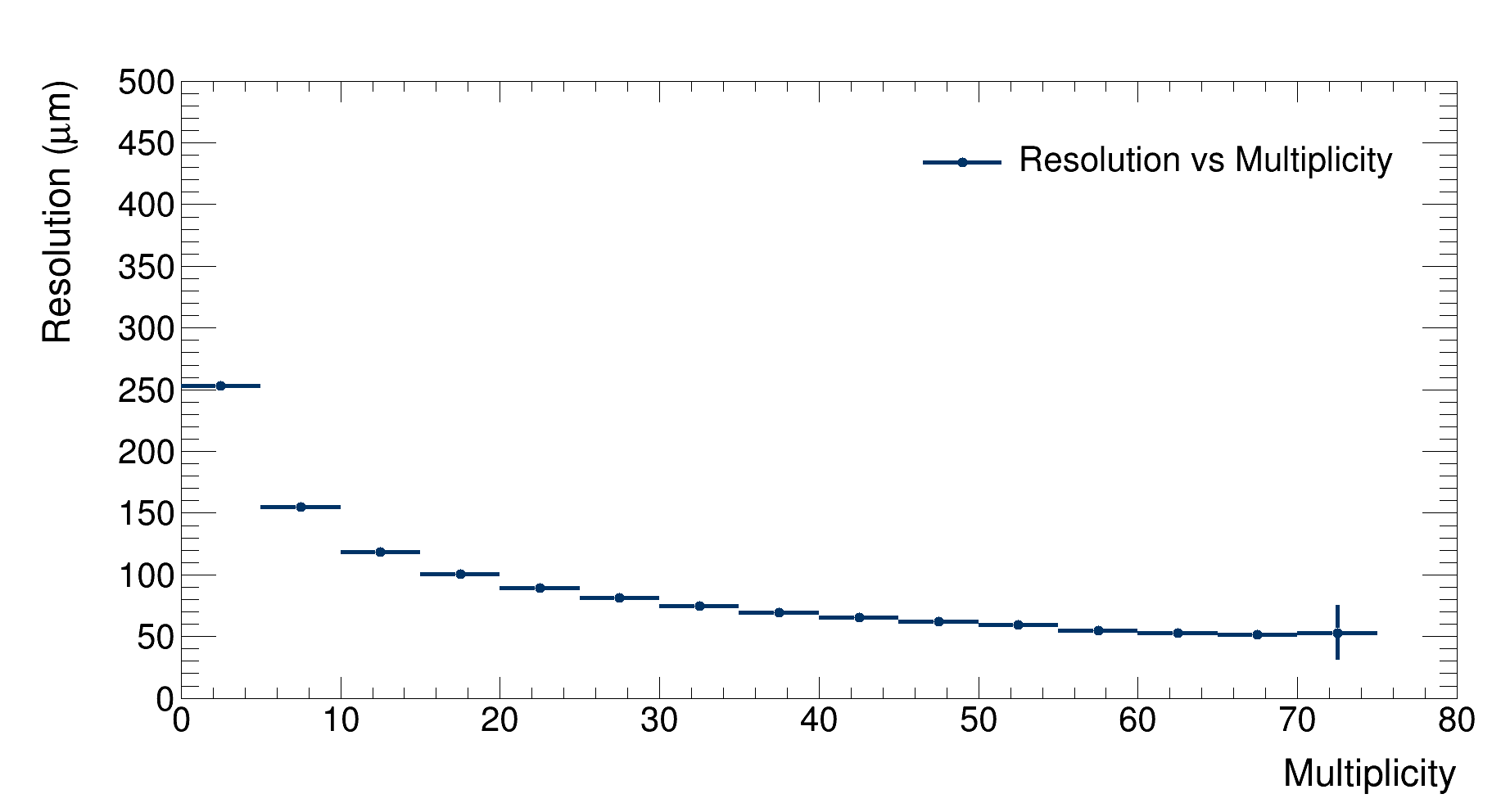 |
|---|
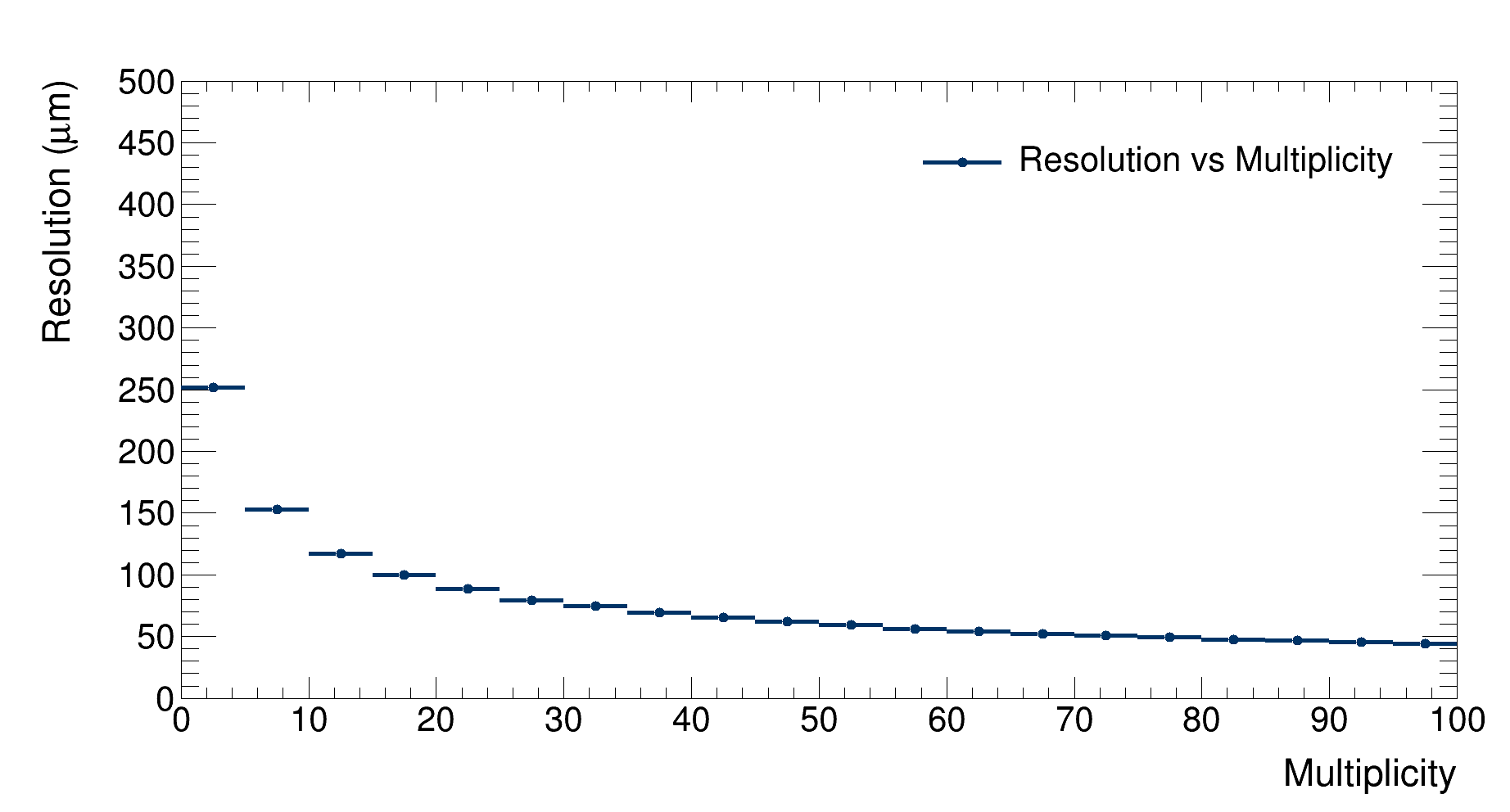
| Detector’s resolution as a function of multiplicity |
As expected, the resolution decreases as multiplicity grows since more tracklets are available to reconstruct the vertex, getting lower then 100 $\mu $m at the highest multiplicities. An increase in resolution is observed at the highest multiplicity bin, but this is due to fluctuations in the simulation (the number of generated events at such multiplicity is very low, as described by the multiplicity pdf).
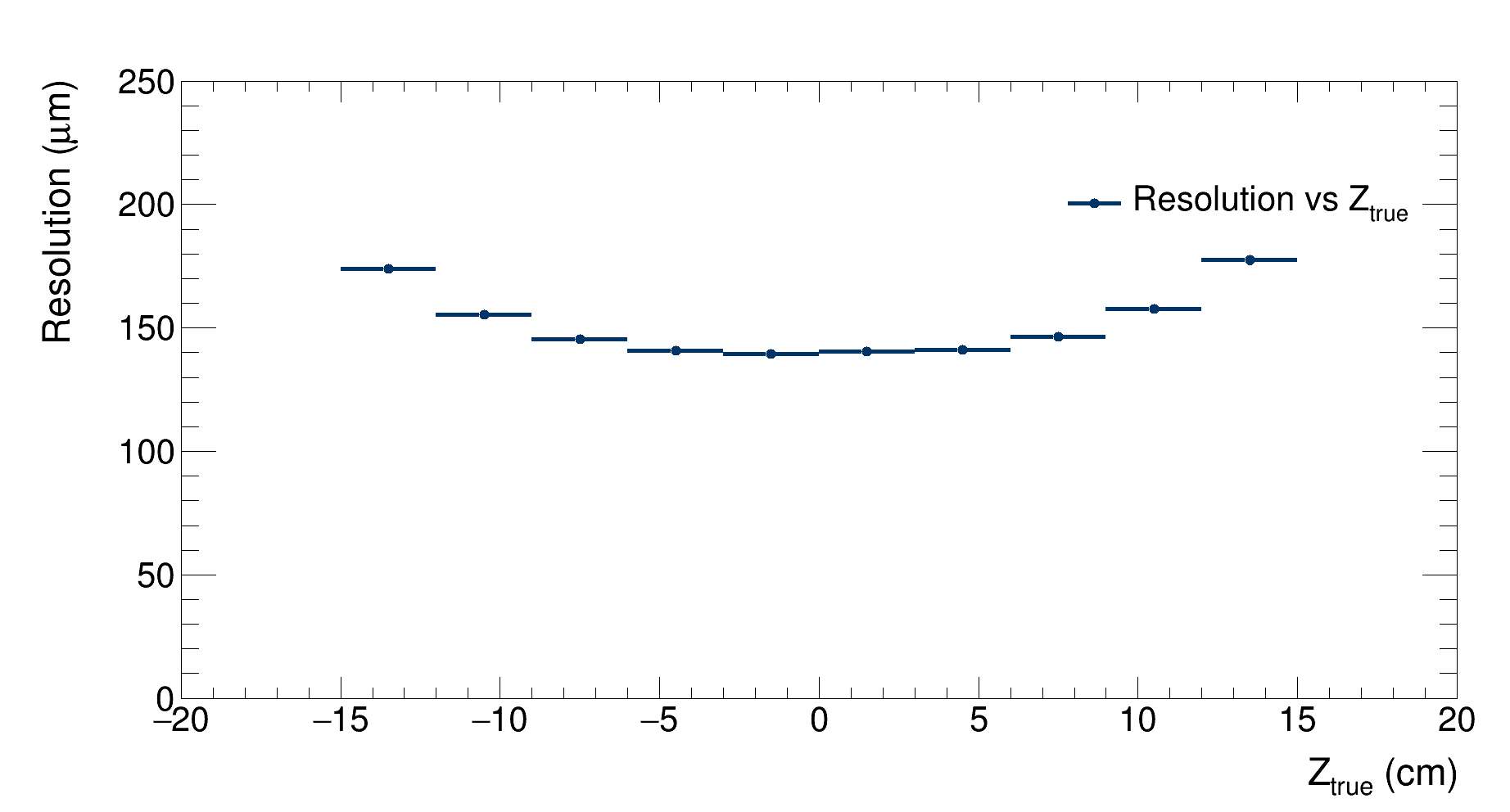 |
|---|
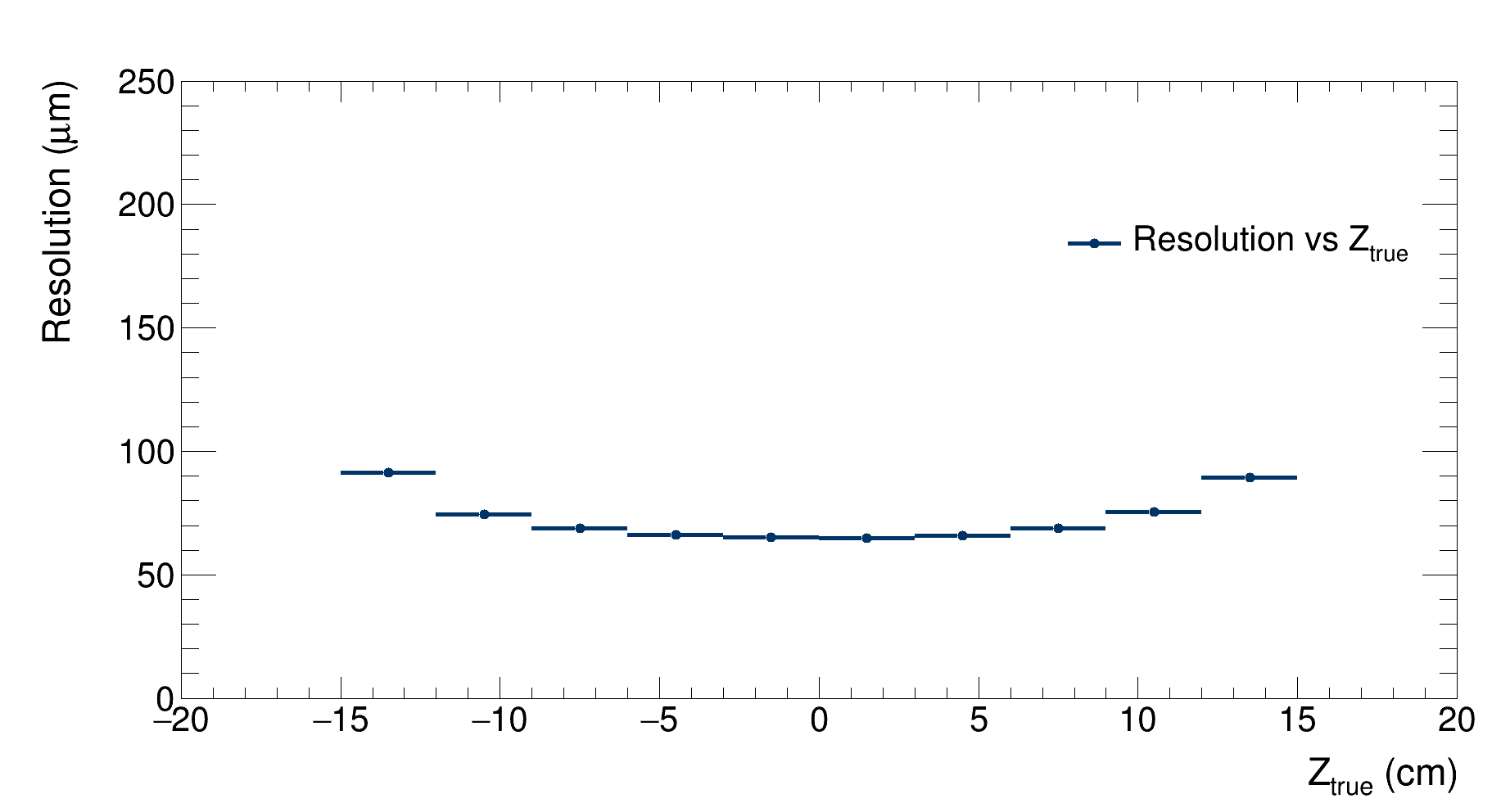
| Detector’s resolution as a function of the Z coordinate of the generated vertex |
As expected, the resolution reaches its minimum when the vertex is generated at the center of the detector, then it grows by 20% up to the point where the vertex is generated outside the detector. In these cases, the resolution grows while the efficiency drops as it is observed in this graph:
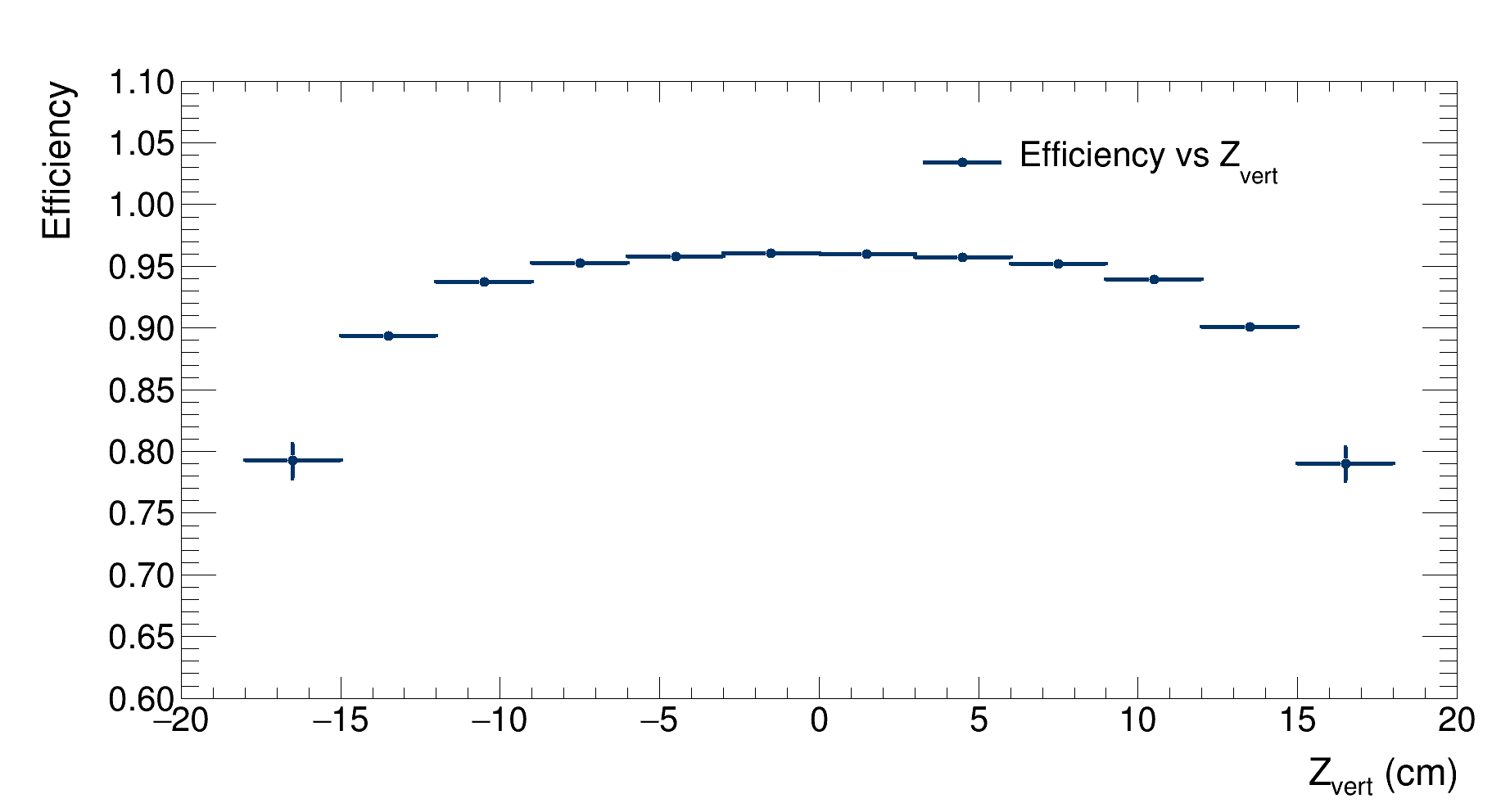 |
|---|
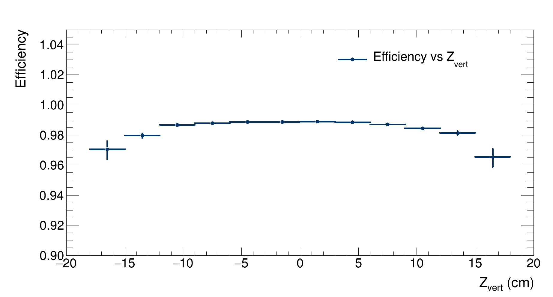
| Detector’s efficiency as a function of the Z coordinate of the generated vertex |
As expected, the efficiency peaks when the vertex is generated at the center of the detector; it then drops when the particles are generated outside the detector.
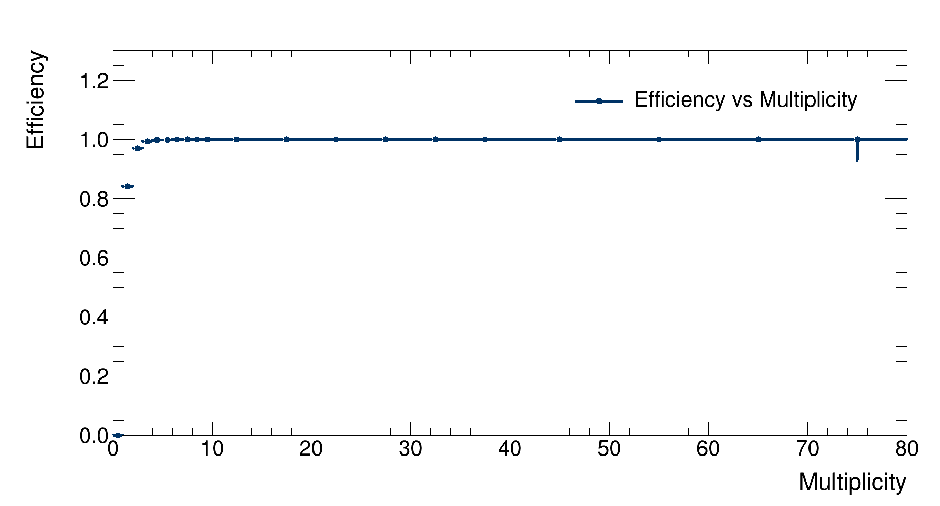 |
|---|
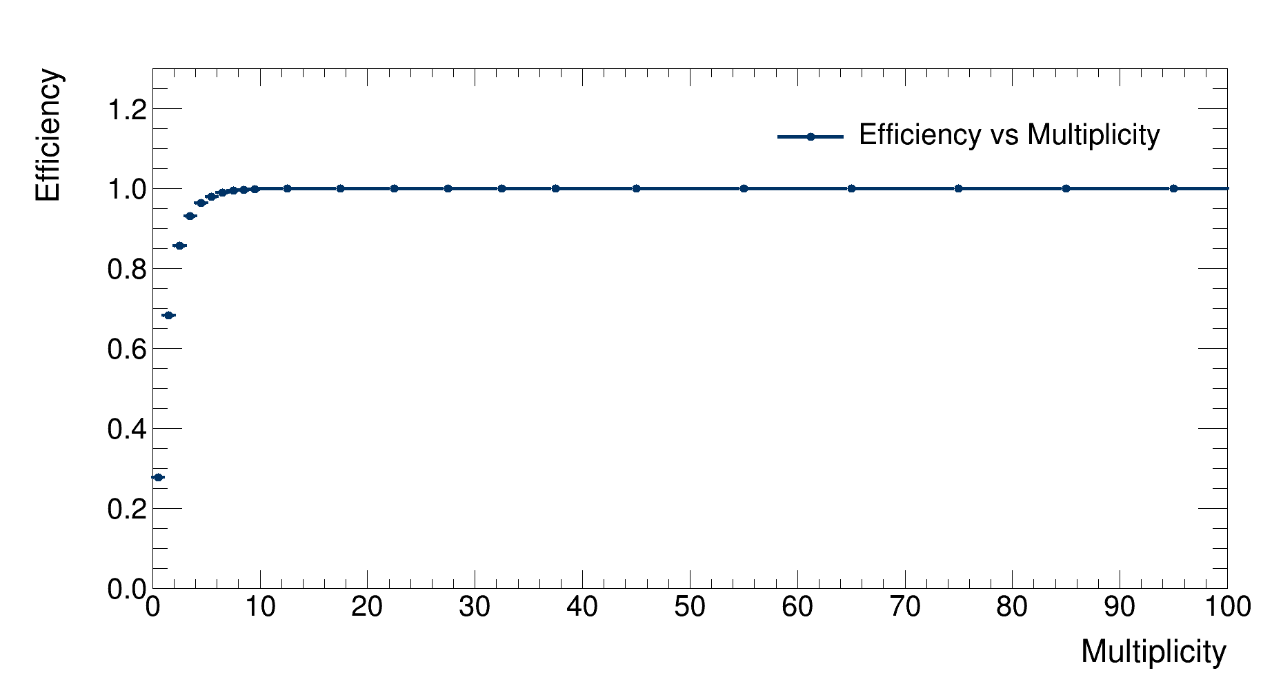
| Detector’s efficiency as a function of the event multiplicity |
As expected, efficiency grows with increasing multiplicity since more tracklets are available to reconstruct the vertex.
❯ Run 2
Configuration:
- N events: 1 million
- Multiplicity distribution: uniform between 0 and 100
- Angular distribution: http://personalpages.to.infn.it/~masera/tans/tans2018/miscellanea/kinem.root, heta2 histogram
- $Z_{vertex}$ distribution: uniform between $-20$ and $20$ cm from the detector’s centre
- $\sigma_{x}=0.01$ cm, $\sigma_{y}=0.01$ cm, $\sigma_{z}=5.3$ cm
- Beam pipe radius: $3$ cm
- Detectors radii: $4$cm, $7$cm
- Mean noise per layer: 10
- MaxPhi: 0.01 mrad
- nSigmaZ: 1
Simulation configuration file here. Reconstruction configuration file here.
Simulation
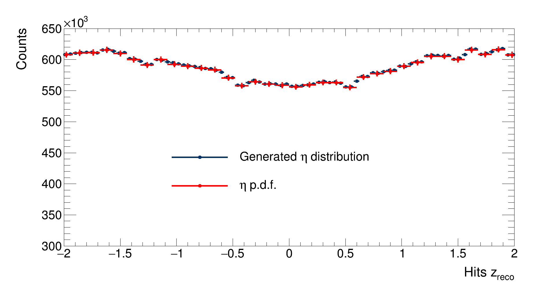
Firstly, the simulated $\eta$ distribution is compared to the desired $\eta$ distribution:
 |
|---|
| Comparison between the simulated $\eta$ distribution and the $\eta$ distribution probability function |
The simulated $\eta$ distribution is scaled with respect to the events of the run. A good agreement between the two distributions is observed. Major differeces between the $Z_{vertex}$ distributions and the $Z$ coordinates of the hits on the layers due to multiple scattering are not observed.
Reconstruction
After the simulation finishes, vertexes are reconstructed and the resolution and efficiency of the detector are evaluated as a function of the event multiplicity and of the event’s vertex $Z$ coordinate.
 |
|---|
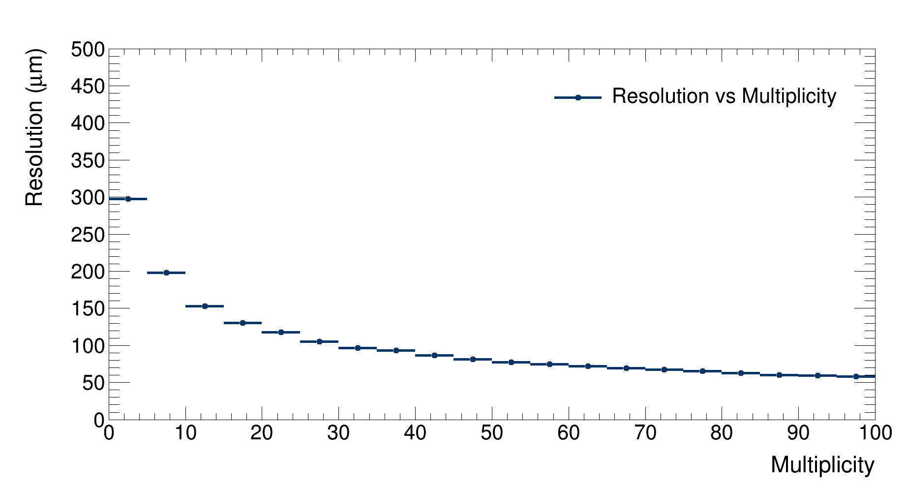
| Detector’s resolution as a function of multiplicity |
As expected, the resolution decreases as multiplicity grows since more tracklets are available to reconstruct the vertex, getting lower then 100 $\mu $m at the highest multiplicities.
 |
|---|
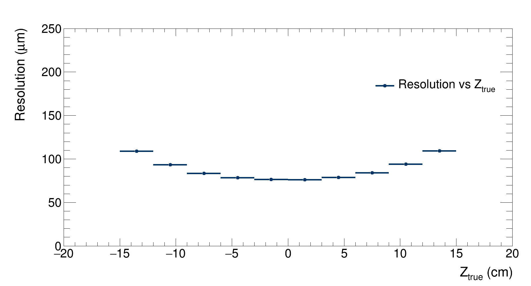
| Detector’s resolution as a function of the Z coordinate of the generated vertex |
As expected, the resolution reaches its minimum when the vertex is generated at the center of the detector, then it grows as vertexes are generated closer to the detectors’ edges. In these cases, the resolution grows while the efficiency drops as it is observed in this graph:
 |
|---|
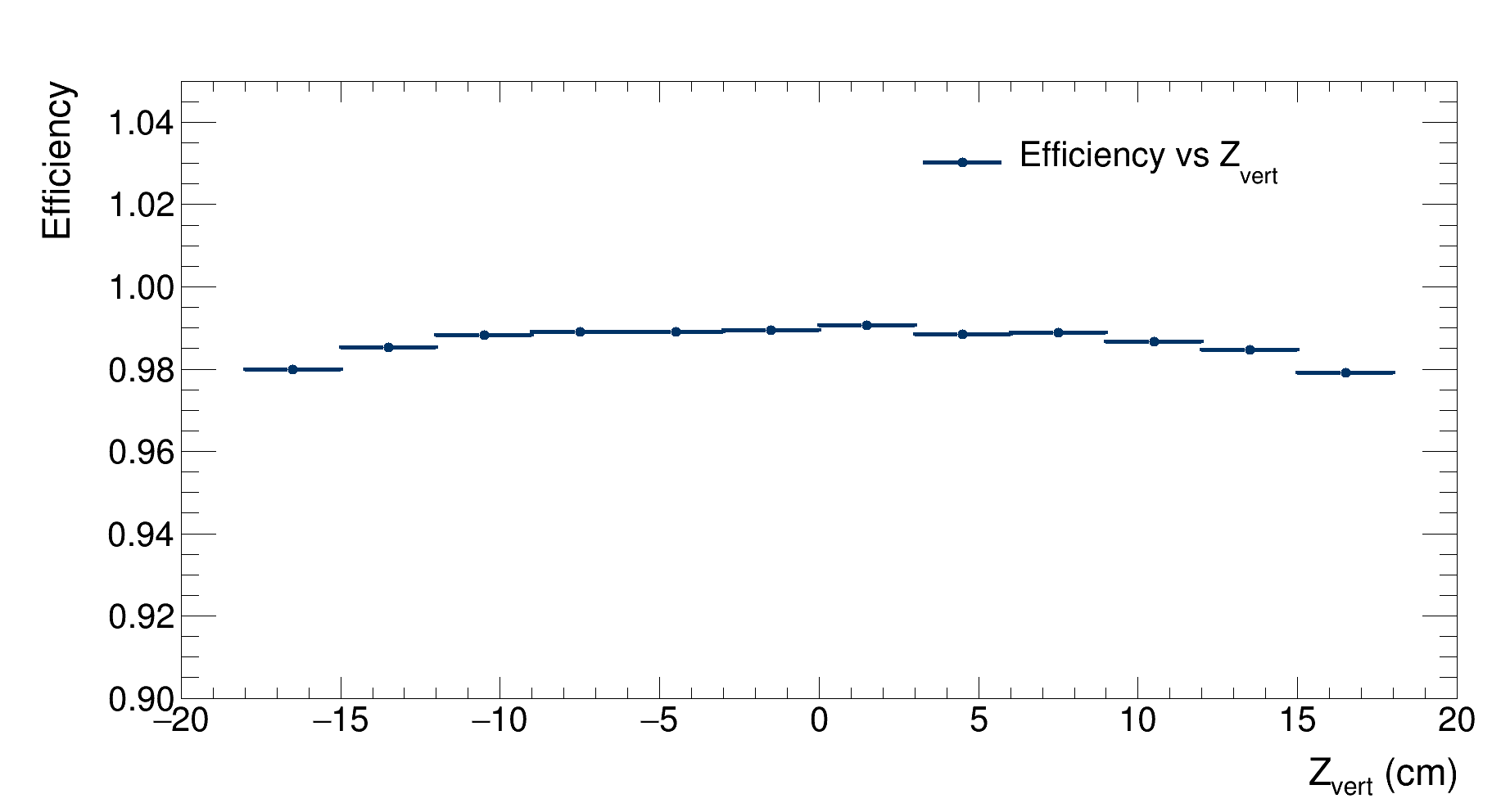
| Detector’s efficiency as a function of the $Z$ coordinate of the generated vertex |
As expected, the efficiency peaks when the vertex is generated at the center of the detector; it then drops when the particles are generated outside the detector.
 |
|---|
| Detector’s efficiency as a function of the event multiplicity |
As expected, efficiency grows with increasing multiplicity since more tracklets are available to reconstruct the vertex.
❯ Run 3
Configuration:
- N events: 1 million
- Multiplicity distribution: uniform between 0 and 100
- Angular distribution: uniform
- $Z_{vertex}$ distribution: gaussian
- $\sigma_{x}=0.01$ cm, $\sigma_{y}=0.01$ cm, $\sigma_{z}=5.3$ cm
- Beam pipe radius: $3$ cm
- Detectors radii: $4$cm, $7$cm
- Noise: no
- MaxPhi: 0.01 mrad
- nSigmaZ: 3
Simulation configuration file here. Reconstruction configuration file here.
Simulation
Multiplicity, angular and $Z_{vertex}$ distributions’ settings differ from the previous runs to cover another case with the aim of comparing the obtained results.
Reconstruction
After the simulation finishes, vertexes are reconstructed and the resolution and effeciency of the detector are evaluated as a function of the event multiplicity and of the event’s vertex $Z$ coordinate.
 |
|---|
| Detector’s resolution as a function of multiplicity |
As expected, the resolution decreases as multiplicity grows since more tracklets are available to reconstruct the vertex, getting lower then 100 $\mu $m at the highest multiplicities.
 |
|---|
| Detector’s resolution as a function of the Z coordinate of the generated vertex |
As expected, the resolution reaches its minimum when the vertex is generated at the center of the detector, then it grows then it grows as vertexes are generated closer to the detectors’ edges. In these cases, the resolution grows while the efficiency drops as it is observed in this graph:
 |
|---|
| Detector’s efficiency as a function of the Z coordinate of the generated vertex |
As expected, the efficiency peaks when the vertex is generated at the center of the detector; it then drops when the particles are generated outside the detector. Lastly, we evaluate efficiency as a function of generated multiplicity:
 |
|---|
| Detector’s efficiency as a function of the event multiplicity |
As expected, efficiency grows with increasing multiplicity since more tracklets are available to reconstruct the vertex.
❯ Comparisons
The results obtained from the different simulations were compared, in order to observe how the different configurations affect the detector’s performance.
Efficiency
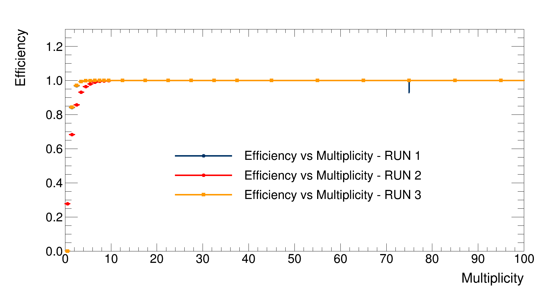
Firstly, the efficiencies as a function of the event multiplicity are compared:
 |
|---|
| Detector’s efficiency vs event multiplicity comparison |
As expected, since the first and the third simulations only differ in the multiplicity distribution, their efficiency distributions overlap. In contrast, since the second simulation has a different $Z_{vertex}$ distribution (uniformly distributed throughout the detector), and since the detector’s efficiency is lower at the edges than at the center, the efficiency for the second simulation is lower.
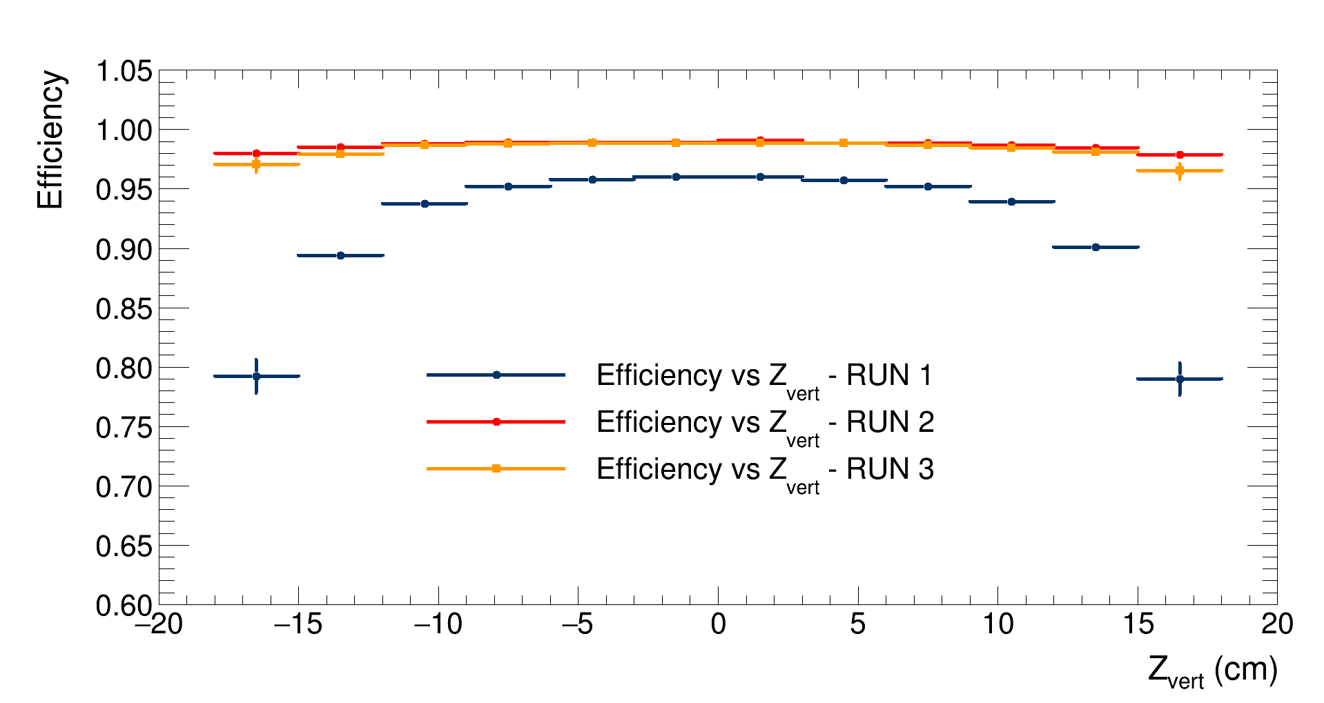
The comparison between the efficiencies as a function of the $Z_{vertex}$ is reported here:
 |
|---|
| Detector’s efficiency vs $Z_{vertex}$ comparison |
As expected, since the first simulation has a multiplicity distribution which is peaked a low multiplicities, where the detector’s efficiency is lower, the resulting efficiency vs $Z_{vertex}$ distribution is lower than the other two simulations. Furthermore, the efficiency drop at the edges of the detector is more significant for this simulation since the probability of multiple particles hitting the detectors is lower (due to the low multiplicity distribution). The efficiencies for the other two simulations are quite similar; with the one for the second simulation being slightly greater due to the fact that the third simulation has a uniform angular distribution, thus forward and backward particles, which will not be detected, are generated. In contrast, with the custom distribution, only particles with $-2 < \eta < 2$ are produced.
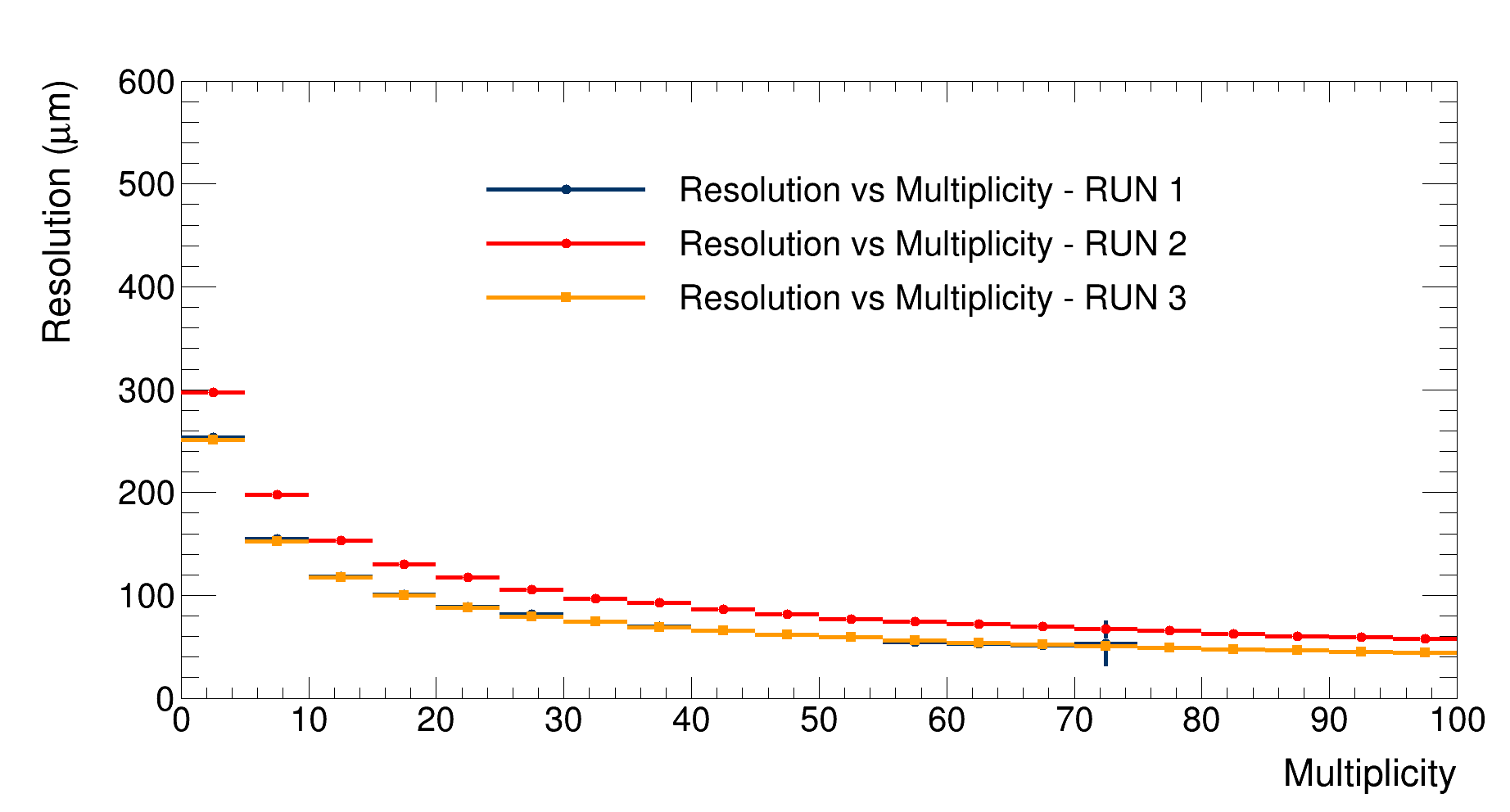
Resolution
 |
|---|
| Detector’s resolution vs event multiplicity comparison |
As expected, the resolution for the second simulation is worse, since more particles are produced close to the detector edges, where the resolution is worse. Since the $Z_{vertex}$ distribution of the other two simulations is the same, their resolution vs $Z_{vertex}$ distribution is similar. We observe a slight difference in the first bins, which is likely due to the gradient of the custom multiplicity distribution within each bin, resulting in a more significant contribution of the low multiplicities in the bins range. The differences observed at higher multiplicities are instead likely due to fluctuations of the first simulation’s stastics, which is limited in this range.
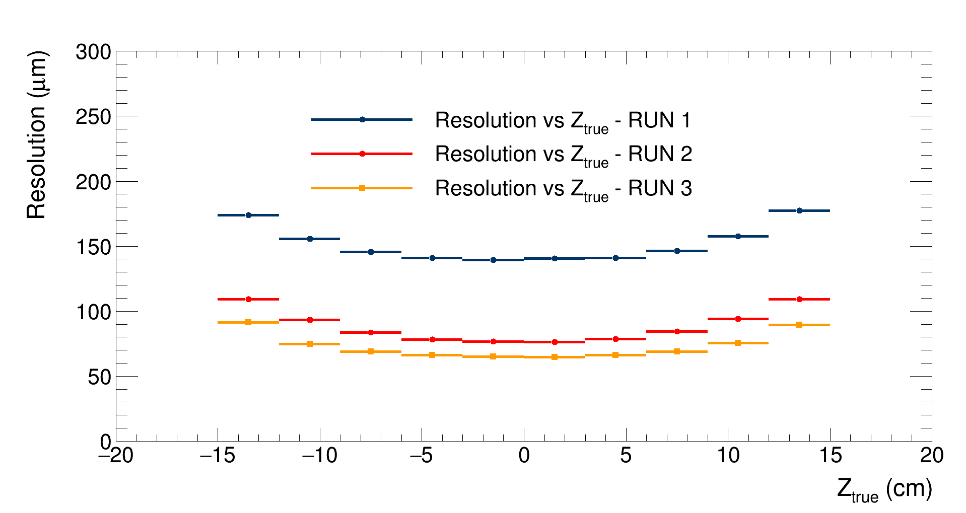
The comparison of the detector’s efficiency vs $Z_{vertex}$ is reported in this graph:
 |
|---|
| Detector’s efficiency vs $Z_{vertex}$ comparison |
As presumed, the resolution for the first simulation is worse since the multiplicity distribution is peaked at low multiplicities, so the number of trackets available to reconstruct the vertex is lower, leading to a worse resolution. The difference between the second and the third simulations is due to the noise, which is activated in the second simulation. The variation of the gap between the two distributions in the different $Z_{vertex}$ bins can be attributed to the fact that the noise is more relevant at the detector’s edges, where the number of particles being detected is lower with respect to events where the collisions happen in the detector’s centre